Introduction
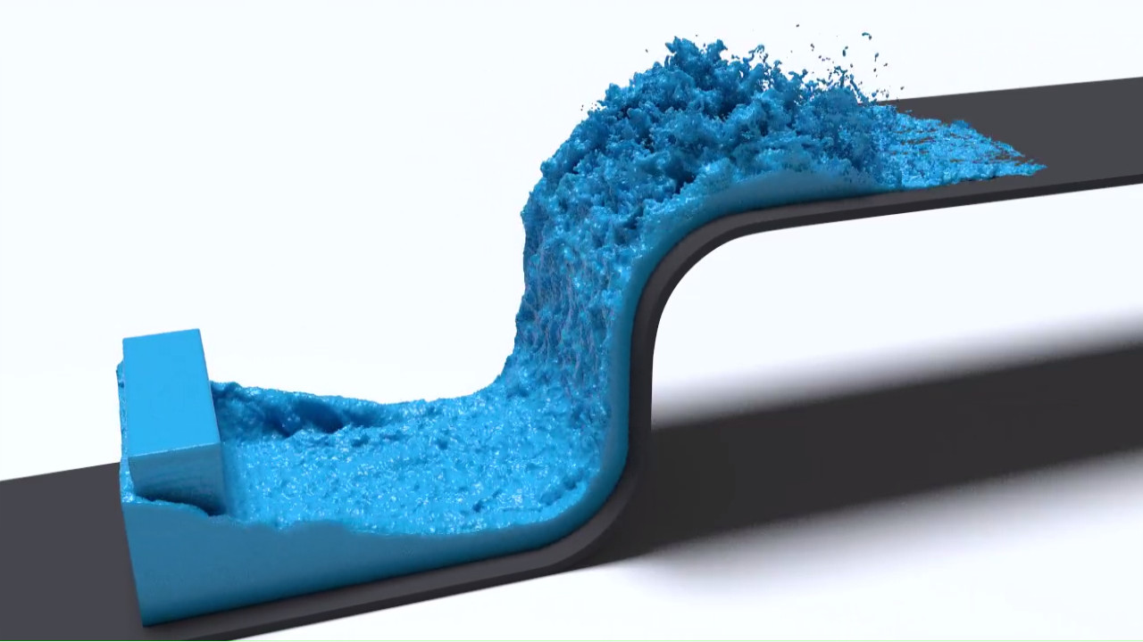
This program is an implementation of a PIC/FLIP liquid fluid simulation written in C++11 based on methods described in Robert Bridson's "Fluid Simulation for Computer Graphics" textbook. The fluid simulation program outputs the surface of the fluid as a sequence of triangle meshes stored in the Stanford .PLY file format which can then be imported into your renderer of choice.
The source code and usage instructions can be found on GitHub.
Features
Below is a list of features implemented in the simulator.
- Isotropic and anisotropic particle to mesh conversion
- Spray, bubble, and foam particle simulation
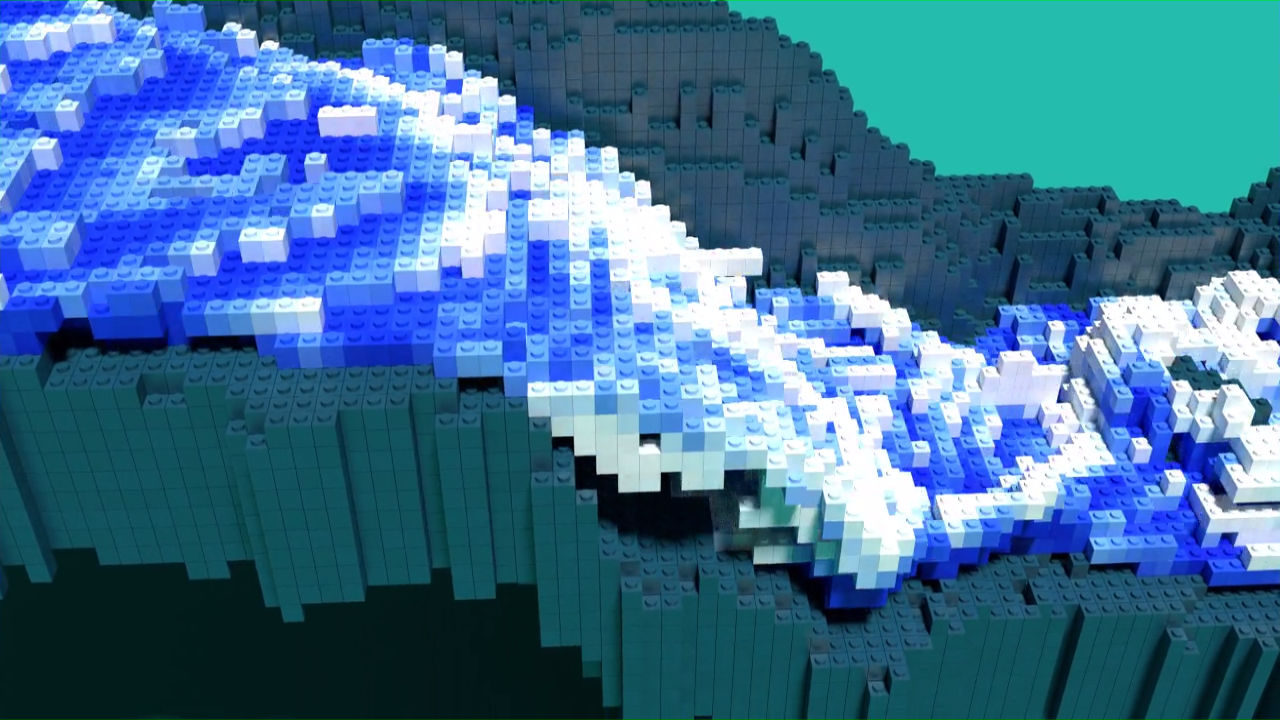
- 'LEGO' brick surface reconstruction
- Save and load state of a simulation
- GPU accelerated tricubic interpolation and fourth-order Runge-Kutta integration using OpenCL
- GPU accelerated velocity advection using OpenCL
- Python bindings
Dependencies
There are three dependencies that are required to build this program:
- OpenCL headers (can be found at khronos.org)
- An OpenCL SDK specific to your GPU vendor (AMD, NVIDIA, Intel, etc.)
- A compiler that supports C++11
Installation
This program uses the CMake utility to generate the appropriate solution, project, or Makefiles for your system. The following commands can be executed in the root directory of the project to generate a build system for your machine:
mkdir build && cd build
cmake ..
Once successfully built, the program will be located in the
build/fluidsim/ directory with the
following directory structure:
fluidsim
│   fluidsim.a      - Runs program configured in main.cpp
│
└───output          - Stores data output by the simulation program
│   └───bakefiles       - meshes
│   └───logs            - logfiles
│   └───savestates      - simulation save states
│   └───temp            - temporary files created by the simulation program
│
└───pyfluid         - The pyfluid Python package
│   └───examples        - pyfluid example usage
│   └───lib             - C++ library files
│
└───resources       - Contains files used during runtime
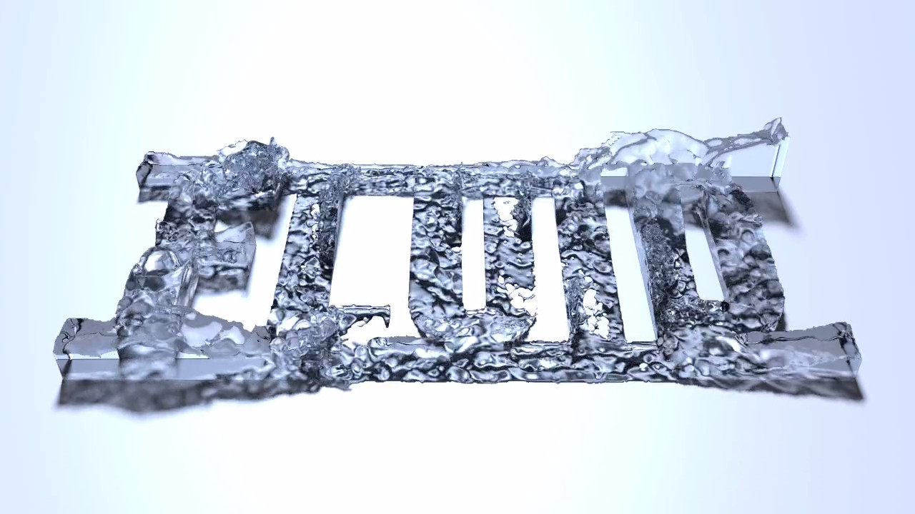
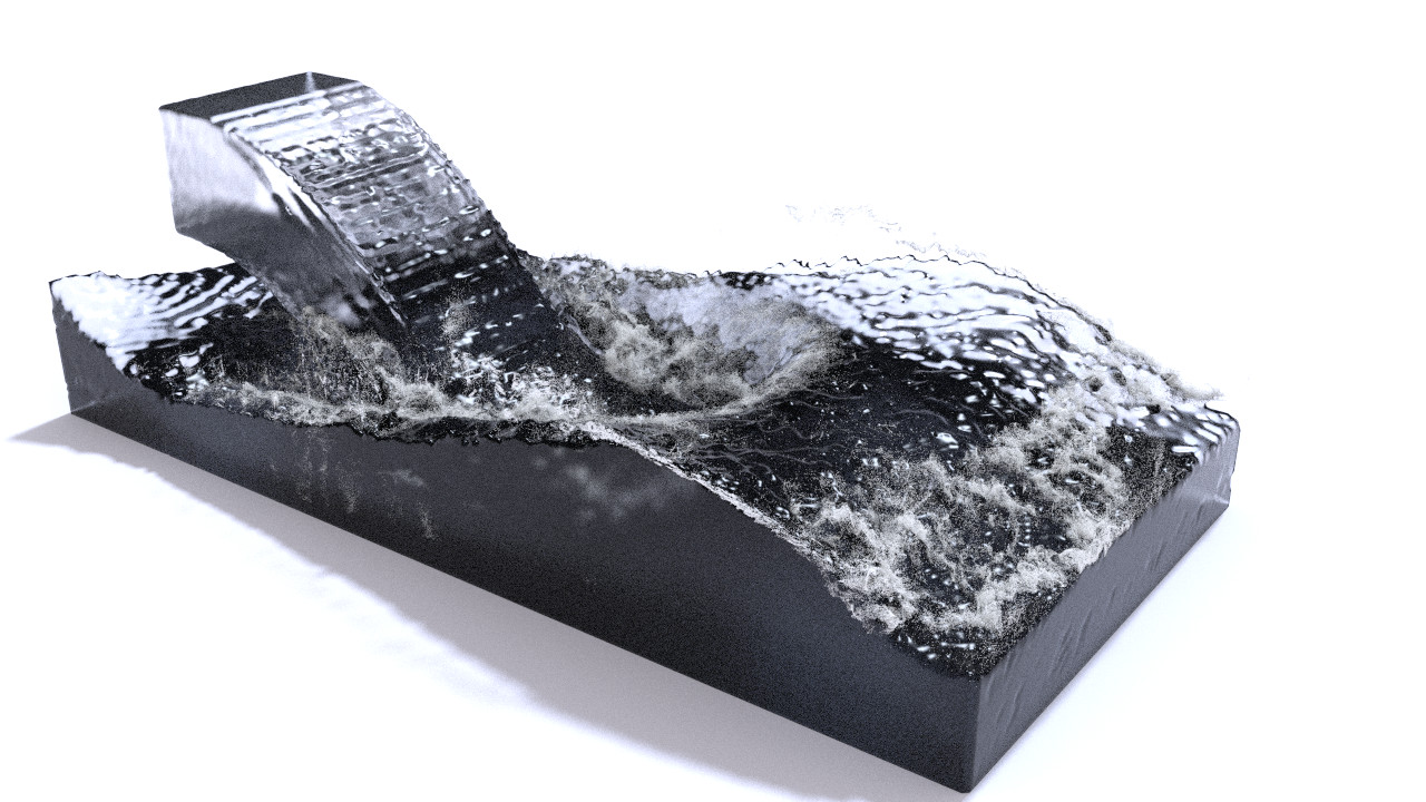
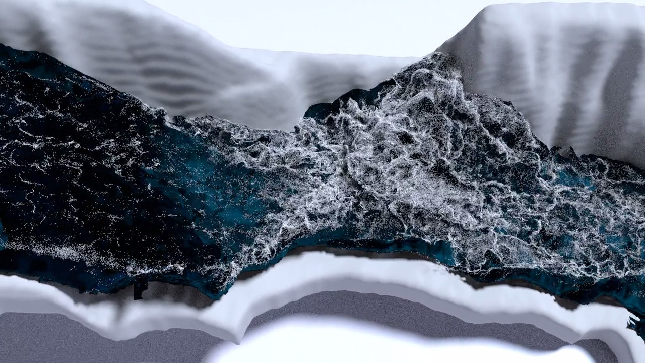
Gallery
The following screencaps are of animations that were simulated within the program and rendered using Blender.


Configuring the Simulator
The fluid simulator can be configured by manipulating a FluidSimulation object in
the function main() located in the file
src/main.cpp.
After building the project, the fluid simulation exectuable will be located in the
fluidsim/ directory. Example configurations are located in the
src/examples/cpp/
directory.
A fluid simulation can also be configured and run within a Python script by importing the
pyfluid package, which will be located in the
fluidsim/ directory after building the project.
Example scripts are located in the
src/examples/python/
directory.
The following two sections will demonstrate how to program a simple "Hello World" simulation using either C++ or Python.
Hello World (C++)
This is a very basic example of how to use the FluidSimulation class to run a simulation. The simulation in this example will drop a ball of fluid in the center of a cube shaped fluid domain. This example is relatively quick to compute and can be used to test if the simulation program is running correctly.
The fluid simulator performs its computations on a 3D grid, and because of this the simulation domain is shaped like a rectangular prism. The FluidSimulation class can be initialized with four parameters: the number of grid cells in each direction \(x\), \(y\), and \(z\), and the width of a grid cell.
int xsize = 32;
int ysize = 32;
int zsize = 32;
double cellsize = 0.25;
FluidSimulation fluidsim(xsize, ysize, zsize, cellsize);
We want to add a ball of fluid to the center of the fluid domain, so we will need to get the
dimensions of the domain by calling getSimulationDimensions and
passing it pointers to store the width, height, and depth values. Alternatively, the
dimensions can be calculated by multiplying the cell width by the corresponding number of
cells in a direction (e.g. width = dx*xsize).
double width, height, depth;
fluidsim.getSimulationDimensions(&width, &height, &depth);
Now that we have the dimensions of the simulation domain, we can calculate the center, and
add a ball of fluid by calling addImplicitFluidPoint which takes
the \(x\), \(y\), and \(z\) position and radius as parameters.
double centerx = width / 2;
double centery = height / 2;
double centerz = depth / 2;
double radius = 6.0;
fluidsim.addImplicitFluidPoint(centerx, centery, centerz, radius);
An important note to make about addImplicitFluidPoint is that it
will not add a sphere with the specified radius, it will add a sphere with half of the
specified radius. An implicit fluid point is represented as a field of values on the
simulation grid. The strength of the field values are 1 at the point center and falls off
towards 0 as distance from the point increases. When the simulation is initialized, fluid
particles will be created in regions where the field values are greater than 0.5. This means
that if you add a fluid point with a radius of 6.0, the ball of fluid in the simulation will
actually be of radius 3.0 since field values will be less than 0.5 at a distance greater than
half of the specified radius.
The FluidSimulation object now has a domain containing some fluid, but the current simulation
will not be very interesting as there are no forces acting upon the fluid. We can add the
force of gravity by making a call to addBodyForce which takes
three values representing a force vector as parameters. We will set the force of gravity to
point downwards with a value of 25.0.
double gx = 0.0;
double gy = -25.0;
double gz = 0.0;
fluidsim.addBodyForce(gx, gy, gz);
Now we have a simulation domain with some fluid, and a force acting on the fluid. Before we
run the simulation, a call to initialize must be made. Note that
any calls to addImplicitFluidPoint must be made before
initialize is called.
fluidsim.initialize();We will now run the simulation for a total of 30 animation frames at a rate of 30 frames per
second by repeatedly making calls to the update function. The
update function advances the state of the simulation by a
specified period of time. To update the simulation at a rate of 30 frames per second, each
call to update will need to be supplied with a time value of 1.0/30.0. Each call to
update will generate a triangle mesh that represents the fluid
surface. The mesh files will be saved in the
fluidsim/output/bakefiles/
directory as a numbered sequence of files stored in the Stanford .PLY file format.
double timestep = 1.0 / 30.0;
int numframes = 30;
for (int i = 0; i < numframes; i++) {
    fluidsim.update(timestep);
}
As this loop runs, the program should output simulation stats and timing metrics to the
terminal. After the loop completes, the
bakefiles/
directory should contain 30 .PLY triangle meshes numbered in sequence from 0 to 29:
000000.ply, 000001.ply, 000002.ply, ..., 000028.ply, 000029.ply
.
If you open the 000029.ply mesh file in a 3D modelling
package such as Blender, the mesh should look similar to
the following image.
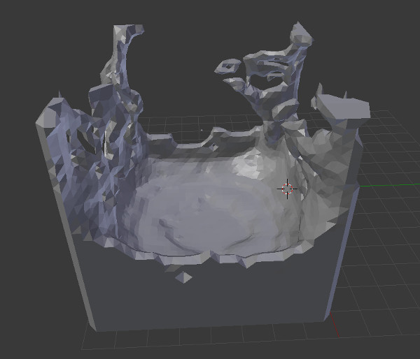
Frame 30 of the Hello World example
The fluid simulation in this example is quick to compute, but of low quality due to the low resolution of the simulation grid. The quality of this simulation can be improved by increasing the simulation dimensions while decreasing the cell size. For example, try simulating on a grid of resolution \(64 {\times} 64 {\times} 64\) with a cell size of \(0.125\), or even better, on a grid of resolution \(128 {\times} 128 {\times} 128\) with a cell size of \(0.0625\).
Hello World (Python)
The following Python script will run the equivalent simulation described in the previous section.
from pyfluid import FluidSimulation

fluidsim = FluidSimulation(32, 32, 32, 0.25)

width, height, depth = fluidsim.get_simulation_dimensions()
fluidsim.add_implicit_fluid_point(width / 2, height / 2, depth / 2, 6.0)
fluidsim.add_body_force(0.0, -25.0, 0.0)
fluidsim.initialize();

for i in range(30):
    fluidsim.update(1.0 / 30)
Program Output
In general, the simulation program will output an animation as a numbered sequence of triangle meshes with each mesh representing the fluid surface at a point in time corresponding to the start of a frame. Some features of the program, when enabled, will output additional files such as colour data or vertex meshes representing a set of particles.
This section will provide details on the structure and organization of the different output files generated by the fluid simulator, and how they can be used in a renderer.
Triangle Meshes and the Stanford .PLY File Format
The program writes triangle meshes in the Stanford .PLY File Format. The .PLY file format was chosen because it is lightweight, simple to implement, and easy to understand. A .PLY file generated by this program is composed of three parts: a header, a list of vertices, and a list of faces.
The header is a series of plaintext lines terminated by a newline character
('\n') that describe the format of the file, vertices, and faces.
The following header describes a binary .PLY file that contains four 3D vertices and two
faces.
ply
format binary_little_endian 1.0
element vertex 4
property float x
property float y
property float z
element face 2
property list uchar int vertex_index
end_header
The vertex list directly follows the end_header line. In the
above header, a vertex element is defined as three floats which represent the x, y, and z
position coordinates.
The face list directly follows the vertex list. A face is made up of some number of vertices
and references individual vertices by an integer index into the previously defined vertex
list. For example, the first vertex in the list would be referenced by the integer
0, the second by 1, and so on. In the
above header, a face element is defined as an unsigned char which denotes the number of
vertices that make up the face followed by a list of integer indices referencing the
vertices. If the mesh is composed of only triangles, then the unsigned char value will be
0x3 for each face. The order of vertices referenced in a face is
important. The .PLY meshes generated by this program do not contain normals, so the left-hand
rule convention of listing the vertices in clockwise order will be used so that the direction
of the faces can be derived from the vertex ordering.
A Simple .PLY Example
This simple .PLY example will demonstrate how the following diagram of a tetrahedron can be converted into a .PLY mesh.
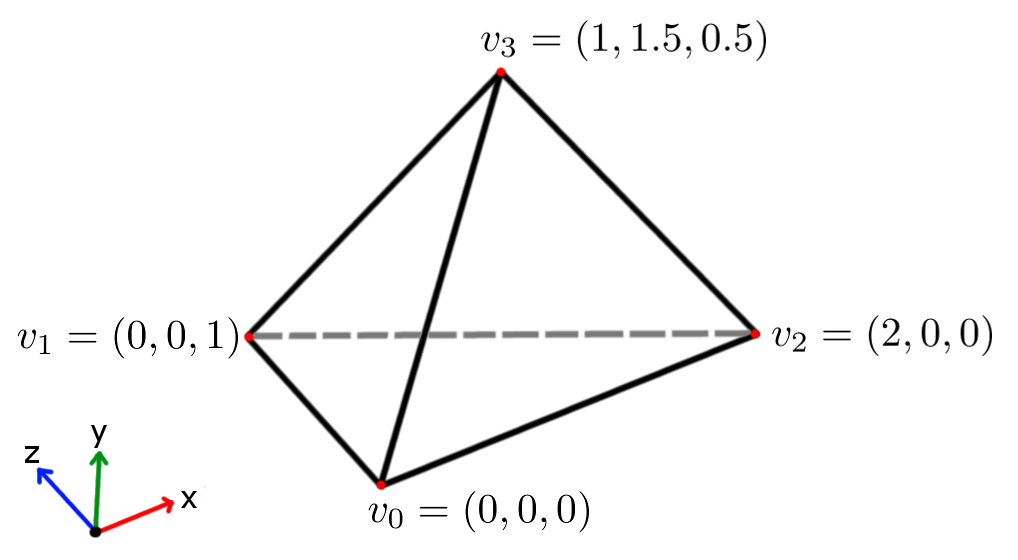
The above tetrahedron is made up of four vertices: \(v_0\), \(v_1\), \(v_2\), and \(v_3\). The vertices can be arranged to create four triangles that make up the faces of the tetrahedron: \(\Delta v_0v_2v_1\), \(\Delta v_0v_1v_3\), \(\Delta v_0v_3v_2\), and \(\Delta v_1v_2v_3\). By modifying the header in the previous section to contain four vertices and four faces, and by listing the vertices and faces in this example, we get the following .PLY file:
ply
format binary_little_endian 1.0
element vertex 4
property float x
property float y
property float z
element face 4
property list uchar int vertex_index
end_header
0 0 0
0 0 1
2 0 0
1 1.5 0.5
3 0 2 1
3 0 1 3
3 0 3 2
3 1 2 3
Remember that the above .PLY format will be written as a binary file, so the header will be stored as chars, the vertices will be stored as floats, the face vertex counts will be stored as unsigned chars, and the face vertex references will be stored as ints. Download the binary .PLY example here.
Isotropic Surface Mesh Output
Isotropic triangle meshes are the default form of program output. These triangle meshes
represent the surface of the fluid and are constructed by the fluid simulator from a set of
spheres with uniform radius. The meshes are written to the
bakefiles/ directory as a sequence of .PLY files in the form
000000.ply, 000001.ply, 000002.ply, ..., where the file
numbers correspond to the frame number.
This type of program output can be used by a renderer to generate renders the fluid surface.
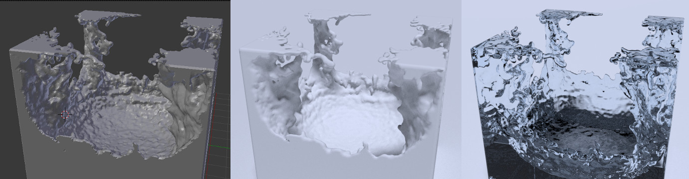
Surface meshes in Blender. Left: Scene view. Middle: Opaque rendering. Right: Transparent rendering.
Anisotropic Surface Mesh Output
Anisotropic triangle meshes represent the surface of the fluid and are similar to isotropic meshes except that the meshes are constructed from a set of ellipsoids instead of a set of spheres. The benefit of constructing the surface from a set of ellipsoids rather than a set of spheres is that sharp/smooth features of the fluid surface are better preserved. This benefit comes at the cost of a longer surface mesh computation time.
The anisotropic meshes are written to the bakefiles/ directory
as a sequence of .PLY files prefixed with the keyword
anisotropic in the form
anisotropic000000.ply, anisotropic000001.ply, anisotropic000002.ply,
            ...
, where the file numbers correspond to the frame number.
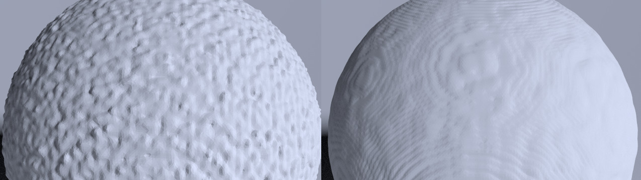
Isotropic vs. anisotropic surface reconstruction. Left: Isotropic. Right: Anisotropic.
Diffuse Particle Output
The diffuse particle feature is a post-processing simulation run ontop of the PIC/FLIP fluid simulation that generates spray, bubble, and foam particles. These diffuse particles can be combined with a surface mesh in a render to give the fluid highly detailed small-scale aeration effects. The diffuse particles are stored as vertex only .PlY meshes where each vertex represents a single diffuse particle.
The diffuse particle meshes are written to the bakefiles/
directory as a sequence of .PLY files prefixed with the keyword
diffuse in the form
diffuse000000.ply, diffuse000001.ply, diffuse000002.ply, ...,
where the file numbers correspond to the frame number.
The simulation program can be configured to sort the diffuse particles by type (spray, foam, or
bubble) and write the output into multiple files per frame. In this case, the files will be
written in the form bubble000000.ply, foam000000.ply,
spray000000.ply, bubble000001.ply, foam000001.ply, spray000001.ply, ....
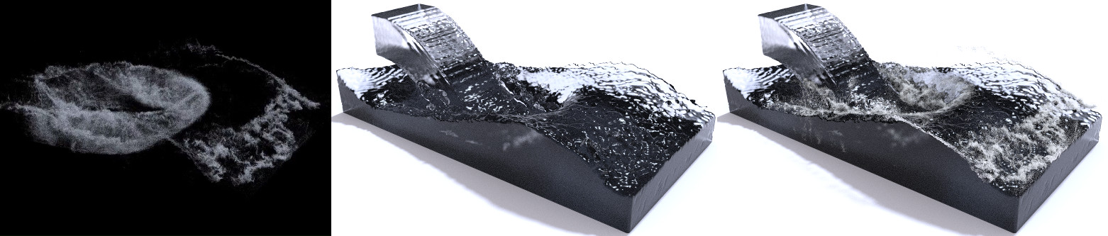
Diffuse Particle Output. Left: Diffuse particles. Middle: Surface mesh. Right: Combined.
LEGO Brick Output
LEGO brick output reconstructs the fluid surface as a set of coloured LEGO bricks. This simulation feature outputs multiple files for each frame that representing LEGO brick locations and multiple formats for representing brick colours. The colour of a brick is a 1-dimensional value on a range of low density to high density.
The colour value of a brick is meant to be used as an input into a gradient within a renderer or shader. For example, a gradient that maps low colour values to white and high colour values to blue can give the illusion of aerated white-water for areas where bricks have a lower density.

Surface vs. LEGO brick surface recontruction. Left: Surface mesh. Right: LEGO brick mesh.
Brick Location Meshes
Brick locations are written as .PLY meshes that contain only vertices where each vertex corresponds to the center location of a brick. These vertex only meshes can be imported into a renderer where a model, such as the model of a LEGO brick can be duplicated over each vertex location prior to rendering.
The brick location meshes are written to the bakefiles/
directory as a sequence of .PLY files prefixed with the keyword
brick in the form brick000000.ply,
brick000001.ply, brick000002.ply, ..., where the file numbers correspond to the frame
number.
The vertices in the .PLY meshes generated by this feature contain vertex color data in addition to position data. To modify the .PLY header described in previous sections to contain vertex colours, the red, green, and blue unsigned char properties are added to the vertex definition. The following example .PLY mesh contains three vertices coloured red, green, and blue respectively.
ply
format binary_little_endian 1.0
element vertex 3
property float x
property float y
property float z
property uchar red
property uchar green
property uchar blue
element face 0
property list uchar int vertex_index
end_header
1 0 3 255 0 0
0 0 2 0 255 0
1 2 1 0 0 255
Note that the red, green, and blue channels are stored as unsigned chars while the vertex positions are stored as floats. Download the binary .PLY example here
Since the brick colour values are 1-dimensional, each RGB channel will have the same value and
be on a range from 0 to 255 inclusive
(0x00 to 0xFF).
Not all renderers have the functionality to read vertex colours in this format. The next two sections will discuss the alternative formats that colour data is written in.
Brick Colour List Data
The program also outputs brick colours as a binary data file. These files can be read by a scripting language within a renderer to retrieve colour information.
The brick colour list data files are written to the bakefiles/
directory as a sequence of .data files prefixed with the keyword
brickcolor in the form
brickcolor000000.data, brickcolor000001.data, brickcolor000002.data,
            ...
, where the file numbers correspond to the frame number.
Brick colours are stored in the data file as red, green, and blue unsigned char values listed in the same order as the vertices in the brick location .PLY file. For example, if \(b_i\) is the \(i^{th}\) brick location in the brick mesh, and \(\text{brickcolors}\) is the color list .data file indexed as an array of unsigned chars, then the colours \(R_i\), \(B_i\), and \(G_i\) can be found in the following manner:
$$ {\large \begin{align} R_i = &\ \text{brickcolors}[3i] \\ G_i = &\ \text{brickcolors}[3i + 1] \\ B_i = &\ \text{brickcolors}[3i + 2] \end{align} } $$Since the brick colour values are 1-dimensional, each RGB channel will have the same value and
be on a range from 0 to 255 inclusive
(0x00 to 0xFF).
Not all renderers may preserve the vertex order after importing the .PLY brick location mesh. If vertex order is not preserved, then the colour information will not be able to be recovered from the brick colour list data file. The next section will discuss a data format where vertex ordering is not required to be preserved and where colour information can be derived from a brick vertex location.
Brick Texture Data
This form of colour output stores brick colour information as a flattened 3D array of unsigned chars. These files can be read by a scripting language within a renderer or can be converted into a 2D image texture which can then be used as a colour look-up table by a shader.
The brick colour texture data files are written to the
bakefiles/ directory as a sequence of .data files prefixed
with the keyword bricktexture in the form
bricktexture000000.data, bricktexture000001.data,
            bricktexture000002.data, ...
, where the file numbers correspond to the frame number.
In the simulation program, brick locations are aligned to a 3D grid of dimensions \(N {\times} M {\times} P\). If the simulation domain width, height, and depth dimensions are \(W {\times} H {\times} D\) respectively, and the width, height, and depth dimensions of a brick are \(w {\times} h {\times} d\) respectively, then:
$$ {\large N = \Bigl \lceil \frac{W}{w} \Bigr \rceil, \quad M = \Bigl \lceil \frac{H}{h} \Bigr \rceil, \quad P = \Bigl \lceil \frac{D}{d} \Bigr \rceil } $$If a brick location vertex has a position of \(x\), \(y\), \(z\), then it's 3D grid index \(i\), \(j\), \(k\) can be computed as:
$$ {\large i = \Bigl \lfloor \frac{x}{w} \Bigr \rfloor, \quad j = \Bigl \lfloor \frac{y}{h} \Bigr \rfloor, \quad k = \Bigl \lfloor \frac{z}{d} \Bigr \rfloor } $$
If brick \(b\) has a 3D grid index \(i\), \(j\), \(k\), and \(\text{bricktexture}\) is the color texture .data file indexed as an array of unsigned chars, then the colours \(R\), \(G\), and \(B\) can be found in the following manner:
$$ {\large R = G = B = \text{bricktexture}[i + jN + kNM ] } $$Since the brick colour values are 1-dimensional, each RGB channel will have the same value and
be on a range from 0 to 255 inclusive
(0x00 to 0xFF). The brick texture .data
files contain values for each possible index of the 3D brick grid. The files will only contain
valid data for grid indices derived from brick locations in the .PLY file.
The Fluid Equations
This simulation program animates fluids by approximating the incompressible Navier-Stokes equations:
$$ {\large \begin{align} \frac{D\vec{u}}{Dt} + \frac{1}{\rho}\nabla p = & \vec{g} + \nu \nabla \cdot \nabla \vec{u}, \\[1.5ex] \nabla \cdot \vec{u} = & 0 \end{align} } $$Where \(\vec{u}\) is velocity, \(\rho\) is the fluid density, \(p\) is pressure, \(\vec{g}\) denotes forces acting on the fluid such as gravity, and \(\nu\) is the kinematic viscosity constant.
This simulator does not implement viscosity in the fluid. If we set \(\nu = 0\), then we can drop the viscosity term and the equations become the inviscid incompressible Navier-Stokes equations:
$$ {\large \begin{align} \frac{D\vec{u}}{Dt} + \frac{1}{\rho}\nabla p = & \vec{g}, \\[1.5ex] \nabla \cdot \vec{u} = & 0 \end{align} } $$The \(D\vec{u} / Dt\) term is the velocity material derivative and is shorthand for \(\partial \vec{u} / \partial t + \vec{u} \cdot \nabla \vec{u}\). A material derivative is the time rate of change of a quantity as it moves through a velocity field. The material derivative in this case can be confusing to understand since the quantity being advected though the velocity field is the velocity field itself.
The second equation, \(\nabla \cdot \vec{u} = 0\), is the incompressibility condition. This equation states that the divergence of the velocity field is zero (divergence-free), meaning that at any region within the velocity field, the amount of fluid entering the region must equal the amount of fluid exiting the region.
The inviscid incompressible Navier-Stokes equations above are too complex to be accurately solved in a single step. The equations will be split up into simpler equations through the method of numerical splitting and each equation will be solved seperately and then added together to give an accurate approximation to the fluid equations. The fluid equations will be split into three parts: the advection equation (material derivative), the body forces equation (gravity), and the pressure equation under the constraint of the incompressibility condition.
$$ {\large \begin{align} \frac{D\vec{u}}{Dt} & = 0, \\[1.5ex] \frac{\partial \vec{u}}{\partial t} & = \vec{g}, \\[1.5ex] \frac{\partial \vec{u}}{\partial t} & + \frac{1}{\rho}\nabla p = 0 \quad \textrm{such that} \quad \nabla \cdot \vec{u} = 0 \end{align} } $$The advantage of splitting the fluid equations is that there are very accurate numerical methods for approximating the above equations.
The fluid simulation algorithm will approximate the fluid equations by repeatedly advancing the simulation state by a small timestep \(\Delta t\). First, the velocity field will be initialized by solving the advection equation. Second, the body forces equation will be solved and added to the previously initialized velocity field. Lastly, the pressure equation will be solved in a way that when the pressure is applied to the velocity field, the fluid will become divergence-free.
Notation and Conventions
This section will detail important notation and conventions that will be used in this document.
3D Arrays and Grid Indices
3D arrays are used throughout the program to store data and computation results. To describe a 3D data value, the symbols \(i\), \(j\), and \(k\) will be used as index values in the \(x\), \(y\), and \(z\) directions respectively.
Notation will be needed to specify data quantities that are aligned to a grid. A quantity \(q\) that is located at grid index \((i, j, k)\) will use the subscript notation \(q_{i,\ j,\ k}\). Data may also be aligned to locations halfway between adjacent grid indices, and in this case we will use half-index notation in the quantity subscripts. For example, a quantity \(q\) that is located halfway between cells \((i, j, k)\) and \((i{+}1, j, k)\) will be notated as \(q_{i{+}1/2,\ j,\ k}\).
Unless otherwise stated, multi-dimensional arrays will be assumed to be stored in row-major order so that data will be accessed sequentially in memory when a 3D array is iterated through in the following manner:
for (int k = 0; k < ksize; k++) {
    for (int j = 0; j < jsize; j++) {
        for (int i = 0; i < isize; i++) {
            print(array3D[k][j][i]);
        }
    }
}
3D Vectors
In general, 3D position vectors will be denoted by the symbol \(\vec{x}\) with components \((x, y, z)\), and 3D velocity vectors will denoted by the symbol \(\vec{u}\) with components \((u, v, w)\).
This document will use the convention that the y-axis points vertically upwards and that the x-axis and z-axis point horizontally.
Classes and Data Structures
This section will detail important data structures and classes used in this project.
Array3d
3D multi-dimensional arrays are used throughout the program to store gridded data. The Array3d data structure is a template class that has functionality for manipulating data stored on a grid using 3D grid indices.
Internally, the gridded data is stored as a flat array of items. If the grid has dimensions \(w\), \(h\), and \(d\), and each item has a data size of \(n\) bytes, then the the Array3d data structure will allocate \(n \cdot w \cdot h \cdot d\) bytes of contiguous memory for storing the gridded data. If an item has a grid index of \((i, j, k)\), it will be stored in the flat array at index \(i + jw + kwh\).
MAC Velocity Field
The marker-and-cell (MAC) velocity field is a grid data structure where instead of having all \((u, v, w)\) velocity components located on a grid cell center, they are located on the centers of their respective grid cell faces. We will use the half-index notation discussed in the Notation and Conventions section of this document to describe the location of cell face centers. For example, the velocity component that is located halfway between cells \((i, j, k{-}1)\) and \((i, j, k)\) is the \(w\) component and is notated as \(w_{i,\ j,\ k{-}1/2}\). The following diagram displays how the \(u\), \(v\), and \(w\) velocity components are laid out on the MAC velocity field.
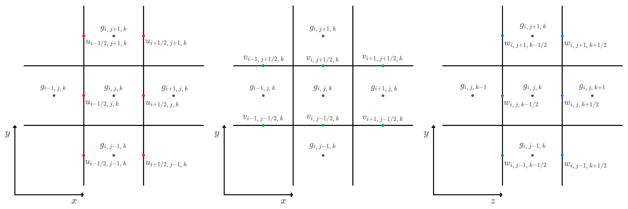
MAC velocity field grid notation diagram.
The advantage of storing velocity components on cell faces rather than storing all components on grid cell centers is that the derivative of the velocity field at cell centers can be approximated very accurately. When velocity components are located on cell faces, the derivative located at the center of cell \(i, j, k\) can be approximated by central differencing:
$$ { \large \begin{align} \left( \frac{\partial u}{\partial x} \right)_{i,\ j,\ k } \approx & \ \frac{u_{i{+}1/2,\ j,\ k} - u_{i{-}1/2,\ j,\ k}}{\Delta x}, \\[1.5ex] \left( \frac{\partial v}{\partial y} \right)_{i,\ j,\ k } \approx & \ \frac{v_{i,\ j{+}1/2,\ k} - v_{i,\ j{-}1/2,\ k}}{\Delta x}, \\[1.5ex] \left( \frac{\partial w}{\partial z} \right)_{i,\ j,\ k } \approx & \ \frac{w_{i,\ j,\ k{+}1/2} - w_{i,\ j,\ k{-}1/2}}{\Delta x} \end{align} } $$Where \(\Delta x\) is the width a grid cell. Accuracy will be needed when calculating velocity field derivatives during the pressure solve stage of the simulation.
The MAC velocity field stores each \(u\), \(v\), and \(w\) velocity component in memory as a seperate Array3d data structure. If the velocity field grid has dimensions \(N {\times} M {\times} P\), then the \(u\) grid will have dimensions \((N {+} 1) {\times} M {\times} P\), the \(v\) grid will have dimensions \(N {\times} (M {+} 1) {\times} P\), and the \(w\) grid will have dimensions \(N {\times} M {\times} (P {+} 1)\).
The half-index notation works well for describing velocity components in this document, but does not translate well into a programming implementation where arrays use integer indexing. The following table demonstrates how half-index notation will be translated into classic array integer indexing:
| Half Index | Integer Index | |
|---|---|---|
| \(\large u_{i{-}1/2,\ j,\ k}\) | \(\large \text{u}(i, j, k)\) | |
| \(\large u_{i{+}1/2,\ j,\ k}\) | \(\large \text{u}(i+1, j, k)\) | |
| \(\large v_{i,\ j{-}1/2,\ k}\) | \(\large \text{v}(i, j, k)\) | |
| \(\large v_{i,\ j{+}1/2,\ k}\) | \(\large \text{v}(i, j+1, k)\) | |
| \(\large w_{i,\ j,\ k{-}1/2}\) | \(\large \text{w}(i, j, k)\) | |
| \(\large w_{i,\ j,\ k{+}1/2}\) | \(\large \text{w}(i, j, k+1)\) |
Evaluating Velocities on the Grid
Evaluating velocities at locations aligned to the grid is straight forward and involves simple averaging of nearby component values. The following formulas will demonstrate how to calculate velocities at points located on the center of grid cells and at points located on cell face centers:
$$ { \begin{align} \vec{u}_{i,\ j,\ k}\ = & \ \left( \frac{u_{i{-}1/2,\ j,\ k} + u_{i{+}1/2,\ j,\ k}}{2}, \ \frac{v_{i,\ j{-}1/2,\ k} + v_{i,\ j{+}1/2,\ k}}{2}, \ \frac{w_{i,\ j,\ k{-}1/2} + w_{i,\ j,\ k{+}1/2}}{2} \right) \\[1.5ex] \vec{u}_{i{+}1/2,\ j,\ k}\ = & \ \left( u_{i{+}1/2,\ j,\ k}, \ \frac{ \begin{align} v_{i,\ j{-}1/2,\ k} \ +& \ v_{i,\ j{+}1/2,\ k} \\\ + \ v_{i{+}1,\ j{-}1/2,\ k} \ +& \ v_{i{+}1,\ j{+}1/2,\ k} \end{align}}{4}, \ \frac{ \begin{align} w_{i,\ j,\ k{-}1/2} \ +& \ w_{i,\ j,\ k{+}1/2} \\ \ + \ w_{i{+}1,\ j,\ k{-}1/2} \ +& \ w_{i{+}1,\ j,\ k{+}1/2} \end{align}}{4} \right) \\[1.5ex] \vec{u}_{i,\ j{+}1/2,\ k}\ = & \ \left( \frac{ \begin{align} u_{i{-}1/2,\ j,\ k} \ +& \ u_{i{+}1/2,\ j,\ k} \\ \ + \ u_{i{-}1/2,\ j{+}1,\ k} \ + & \ u_{i{+}1/2,\ j{+}1,\ k} \end{align}}{4}, \ v_{i,\ j{+}1/2,\ k}, \ \frac{ \begin{align} w_{i,\ j,\ k{-}1/2} \ +& \ w_{i,\ j,\ k{+}1/2} \\ \ + \ w_{i,\ j{+}1,\ k{-}1/2} \ +& \ w_{i,\ j{+}1,\ k{-}1/2} \end{align}}{4} \right) \\[1.5ex] \vec{u}_{i,\ j,\ k{+}1/2}\ = & \ \left( \frac{ \begin{align} u_{i{-}1/2,\ j,\ k} \ +& \ u_{i{+}1/2,\ j,\ k} \\ \ + \ u_{i{-}1/2,\ j,\ k{+}1} \ +& \ u_{i{+}1/2,\ j,\ k{+}1} \end{align}}{4}, \ \frac{ \begin{align} v_{i,\ j{-}1/2,\ k} \ +& \ v_{i,\ j{+}1/2,\ k} \\ \ + \ v_{i,\ j{-}1/2,\ k{+}1} \ +& \ v_{i,\ j{+}1/2,\ k{+}1} \end{align}}{4}, \ w_{i,\ j,\ k{+}1/2} \right) \\[1.5ex] \end{align} } $$Evaluating Velocities off the Grid
Evaluating velocities that are not aligned to grid locations will involve interpolating between nearby grid values. We will use tricubic interpolation to evaluate values not aligned to the grid. A tricubic interpolation will involve weighting 64 points aligned to the vertices of a \(3{\times}3{\times}3\) grid of cubes where the point being evaluated is located inside the center cube. Since velocity components are staggered at different locations on the MAC velocity field, three seperate tricubic interpolations will need to be computed in order to evaluate the velocity at a single point.
The inputs to the tricubic interpolation method will be a 3D array of dimension \(4{\times}4{\times}4\), and three values \(x, y, z \in [0, 1]\) that will define the location within the unit cube that is being interpolated. The \(x, y, z\) values will be located between the indices \((1, 1, 1)\) and \((2, 2, 2)\) in the 3D array of interpolation values.
The following tricubicInterpolate method was adapted from
Paul Bourke's Cubic Interpolation Page.
double cubicInterpolate(double p[4], double x) {
    return p[1] + 0.5 * x*(p[2] - p[0] +
                           x*(2.0*p[0] - 5.0*p[1] + 4.0*p[2] - p[3] +
                              x*(3.0*(p[1] - p[2]) + p[3] - p[0])));
}

double bicubicInterpolate(double p[4][4], double x, double y) {
    double arr[4];
    arr[0] = cubicInterpolate(p[0], x);
    arr[1] = cubicInterpolate(p[1], x);
    arr[2] = cubicInterpolate(p[2], x);
    arr[3] = cubicInterpolate(p[3], x);
    return cubicInterpolate(arr, y);
}

double tricubicInterpolate(double p[4][4][4], double x, double y, double z) {
    double arr[4];
    arr[0] = bicubicInterpolate(p[0], x, y);
    arr[1] = bicubicInterpolate(p[1], x, y);
    arr[2] = bicubicInterpolate(p[2], x, y);
    arr[3] = bicubicInterpolate(p[3], x, y);
    return cubicInterpolate(arr, z);
}
The above method computes a tricubic interpolation by first computing four bicubic interpolations on the \(xy\)-plane and taking a cubic interpolation of the resulting values along the \(z\)-axis. Each bicubic interpolation computes four cubic interpolations along the \(x\)-axis and takes an additional cubic interpolation of the resulting values along the \(y\)-axis. The following cubic spline function is used to compute the cubic interpolations:
$$ { \begin{align} f(p_0,\ p_1,\ p_2,\ p_3,\ x) = \ &(-\tfrac{1}{2}p_0 + \tfrac{3}{2}p_1 - \tfrac{3}{2}p_2 + \tfrac{1}{2}p_3)x^3 \\ &+ (p_0 - \tfrac{5}{2}p_1 + 2p_2 - \tfrac{1}{2}p_3)x^2 \\ &+ (-\tfrac{1}{2}p_0 + \tfrac{1}{2}p_2)x \\ &+ p_1 \end{align} } $$The following methods demonstrate how the above tricubic interpolation method can be used with the MAC velocity field to compute a velocity at any location within the grid:
double evaluateComponentVelocity(Vector3 position,
                                 Vector3 gridOffset,
                                 Array3d grid) {
    position -= gridOffset;
    int gi = floor(position.x / dx);
    int gj = floor(position.y / dx);
    int gk = floor(position.z / dx);

    double points[4][4][4];
    for (int k = 0; k < 4; k++) {
        for (int j = 0; j < 4; j++) {
            for (int i = 0; i < 4; i++) {
                points[k][j][i] = grid(i + gi - 1, j + gj - 1, k + gk - 1);
            }
        }
    }

    Vector3 gpos = Vector3(gi, gj, gk) * dx;
    Vector3 interp = (position - gpos) / dx;

    return tricubicInterpolate(points, interp.x, interp.y, interp.z);
}

Vector3 evaluateVelocityAtPosition(Vector3 position) {
    double hdx = 0.5 * dx;
    Vector3 offsetU(0.0, hdx, hdx);
    Vector3 offsetV(hdx, 0.0, hdx);
    Vector3 offsetW(hdx, hdx, 0.0);

    double vx = evaluateComponentVelocity(position, offsetU, U);
    double vy = evaluateComponentVelocity(position, offsetV, V);
    double vz = evaluateComponentVelocity(position, offsetW, W);

    return Vector3(vx, vy, vz);
}
Where the \(\text{dx}\) variable represents the width of a grid cell, \(\Delta x\), and the \(\text{U}\), \(\text{V}\), and \(\text{W}\), grids are the respective \(u\), \(v\), and \(w\) MAC velocity field component grids.
Note that in the above methods, if the \(\text{position}\) vector is near the edge of the grid, the \(\text{points}\) array may be set to values that are out of range of the component grid. In this program, out of range values are simply set to zero.
Fragmented Vector
The fragmented vector class is a vector-like template class where data is stored in multiple equal sized chunks of contiguous memory. The reason for storing data as a series of contiguous chunks rather than a single contiguous chunk is that some vectors in this simulator may become very large and the program may not be able to allocate a block of memory that is large enough.
For example, a fluid particle consists of a 3D position vector and a 3D velocity vector and if each vector stores its components each as 32-bit floats, then the total size of a fluid particle will be 24 bytes. If a simulation needs to store 30 million fluid particles, a contiguous vector will need to be able to allocate a single 720MB block of memory, which may not be possible, especially if the program memory becomes fragmented. If the 30 million fluid particles are instead stored as 30 chunks of 1 million particles each, the program may have an easier time finding space to store each 24MB block of memory.
The fragmented vector class stores its contents as a vector of vectors where each inner vector is restricted to contain some max number of items. In C++, if the standard template library vector class is used, the vector of vectors will have a type definition of:
std::vector< std::vector<T> > fragmentedVector;
Where T is the data type that the fragmented vector will
store.
If the fragmented vector stores elements of type \(T\), and each inner vector contains a maximum number of elements \(n\), then the \(i^{th}\) element, \(T_i\), can be accessed in the following manner:
$$ { \large T_i = \text{fragmentedVector}[\ \lfloor i / n \rfloor \ ][i \bmod n] } $$Material Grid
A cell within the simulation grid can be in one of three states: fluid, solid, or air. The material grid class is used in the simulation program to track where fluid exists within the simulation grid and to track where solid objects are located. This class also provides useful methods for querying information about the material grid such as whether a face is bordering a certain material type, or whether a cell has a neighbour of certain material type.
The fluid, liquid, and air material types are stored as chars in a C++ class enumeration, and the material type grid is stored in an Array3d data structure:
enum class Material : char {
    air   = 0x00,
    fluid = 0x01,
    solid = 0x02
};

Array3d<Material> materialGrid;
Scalar Field
The scalar field class is used for storing scalar values on a grid in 3D space. Instead of using the convention that gridded values are aligned to grid cell centers, this class uses the convention that scalar values are aligned to the vertices of grid cells. If a 3D grid has dimensions \(W {\times} H {\times} D\) and a cell width of \(\Delta x\), the scalar field will have dimensions \((W{+}1) {\times} (H{+}1) {\times} (D{+}1)\), and a value \(s_{i,\ j,\ k}\) will be located at position \(\vec{x}_{i,\ j,\ k} = (i\Delta x,\ j\Delta x,\ k\Delta x)\).
The scalar field values are stored as floats in an Array3d data structure where all values are initialized to zero.
The scalar field class is used in the advection stage, and the fluid surface reconstruction stage of the fluid simulation. Both stages involve transferring point values to a grid.