Introduction
This program is an implementation of a procedural map generator based upon methods described in Martin O'Leary's "Generating fantasy map" notes. Features include irregular Voronoi grid generation, simulated erosion model, city and border generation, and simulated annealing automated label placement. Written in C++ and drawn using the Cairo graphics library.
This project uses jsoncons for parsing JSON data, Argtable3 for parsing command line arguments, Python and PyCairo for drawing, and data from GeoNames for city name data.
The source code is hosted on GitHub: http://github.com/rlguy/FantasyMapGenerator
Gallery
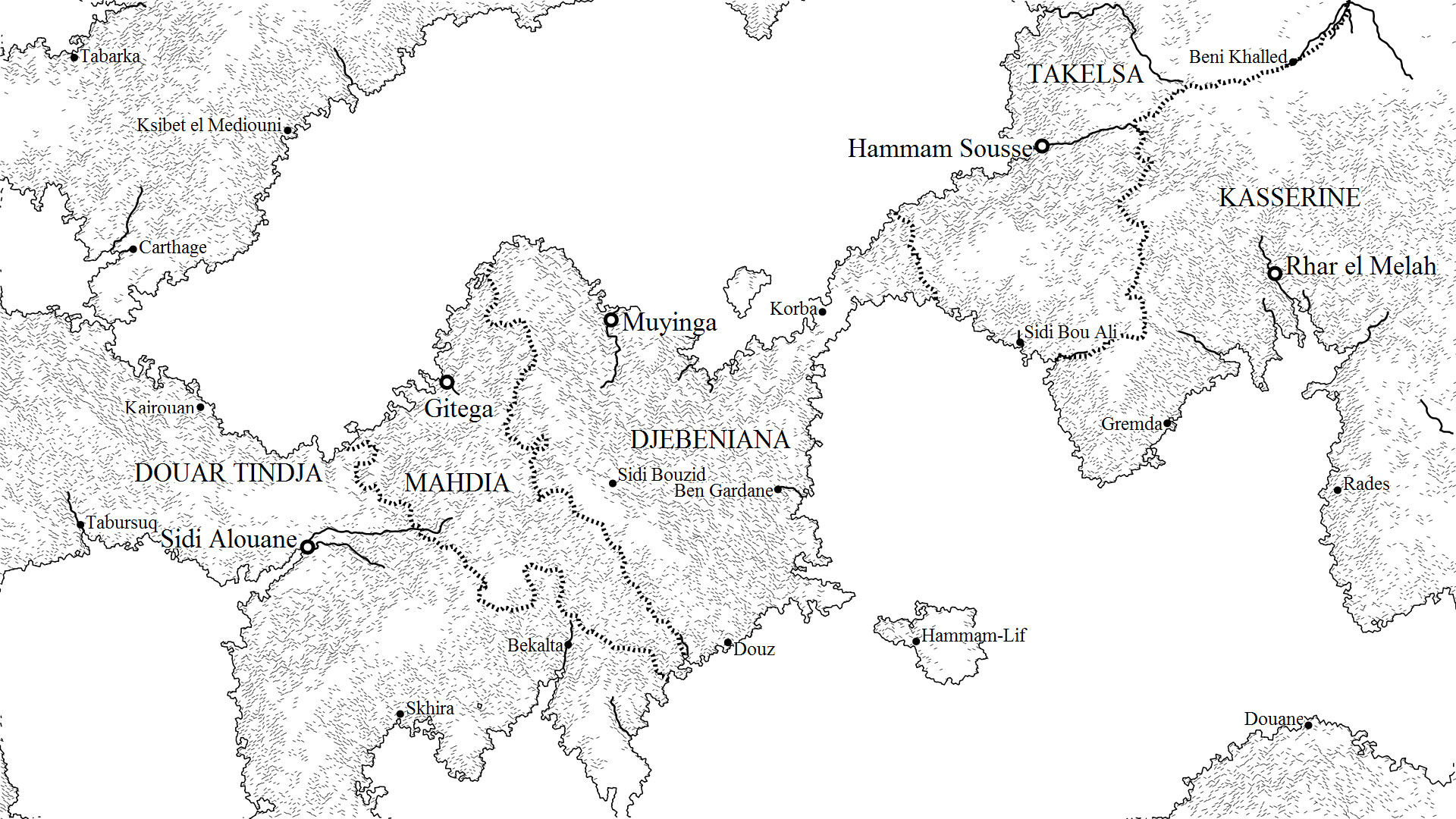
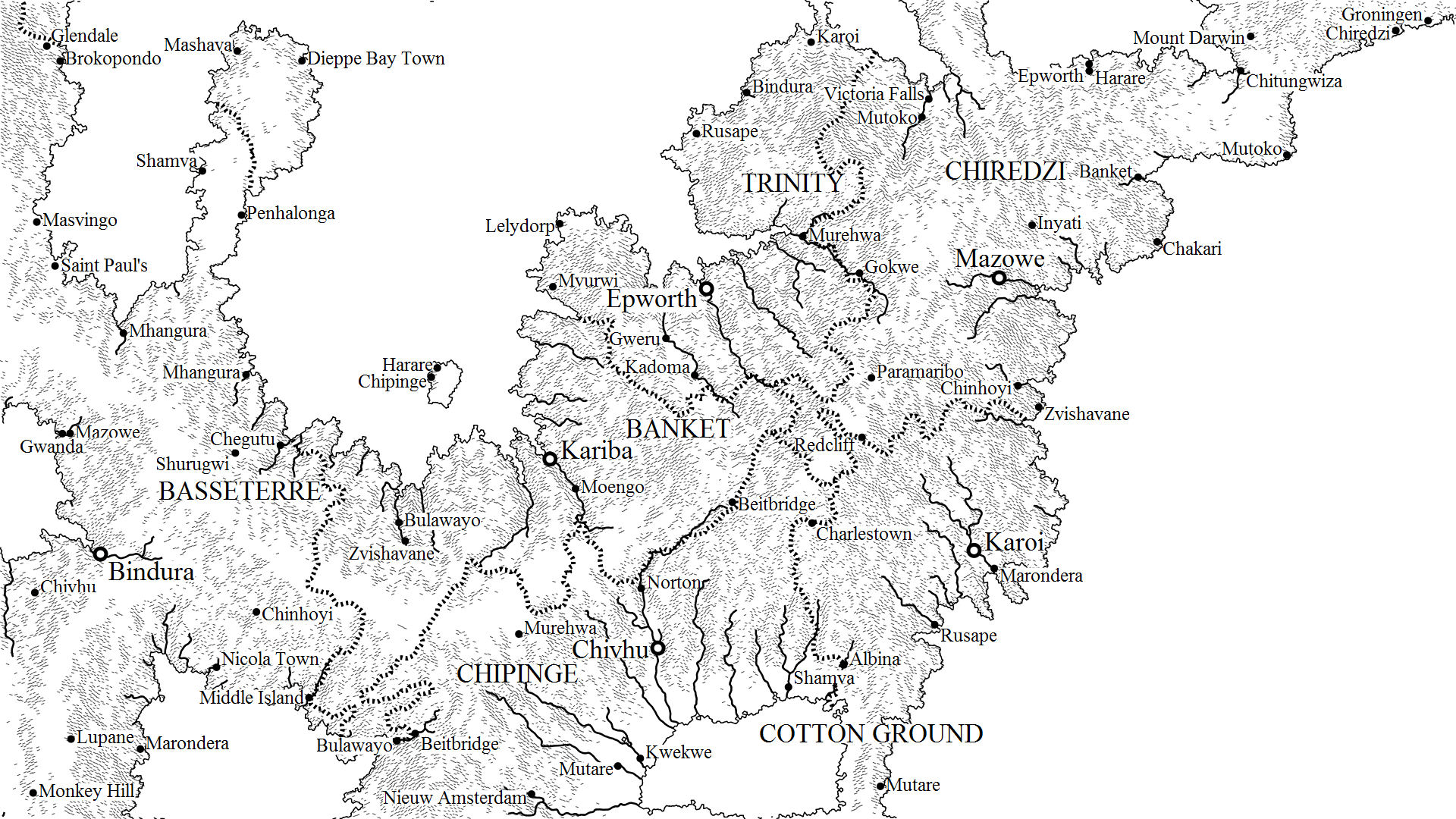
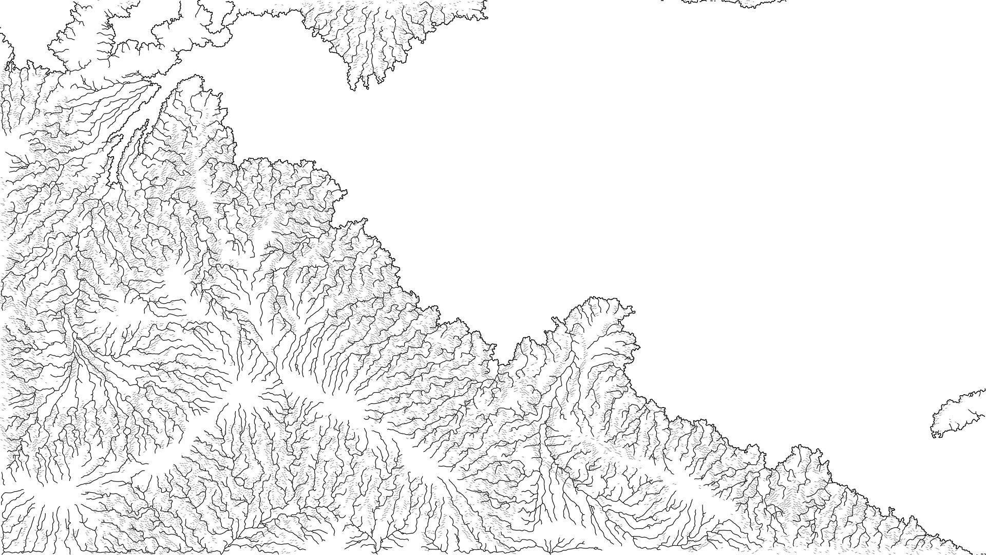
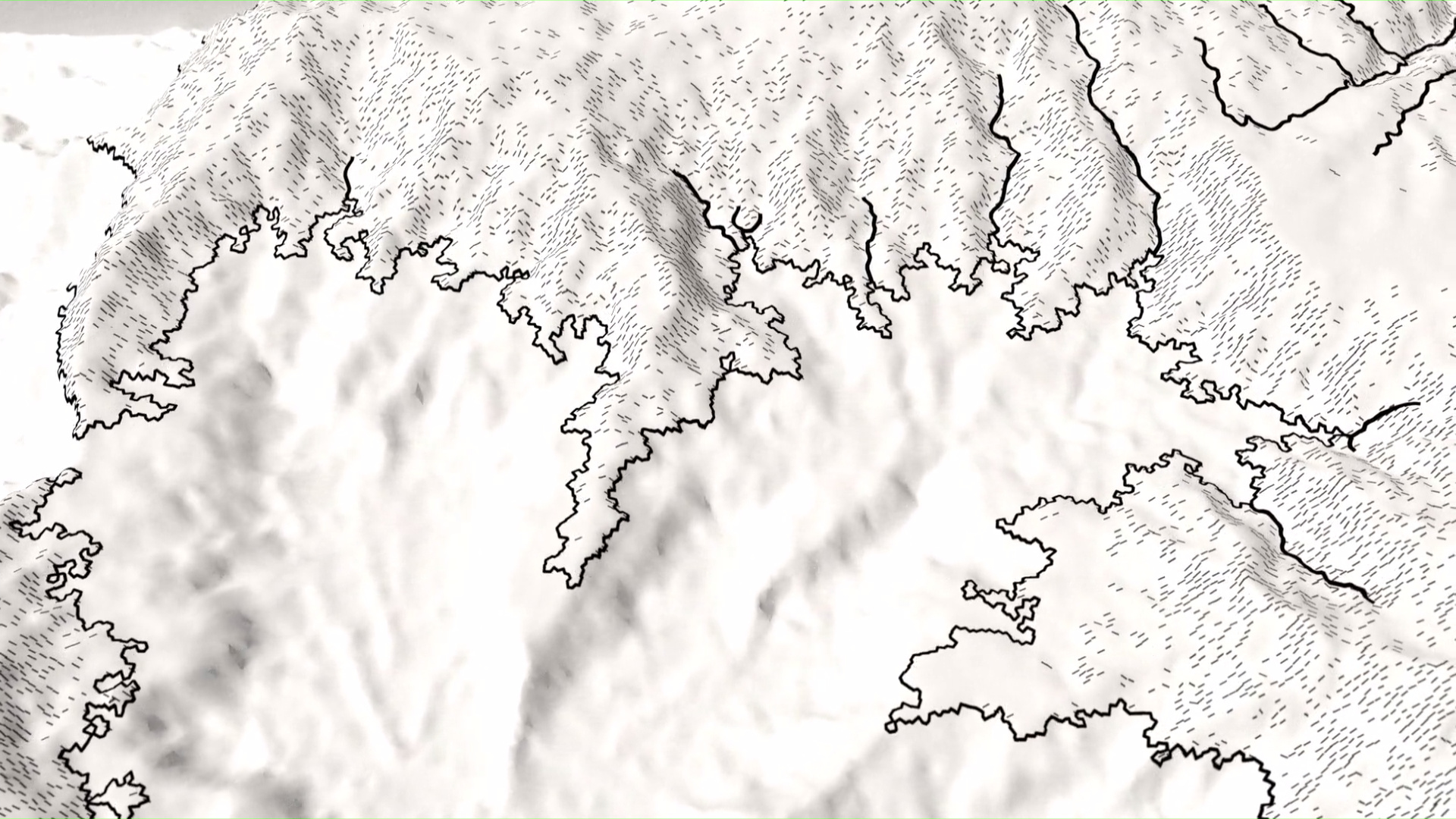
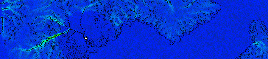
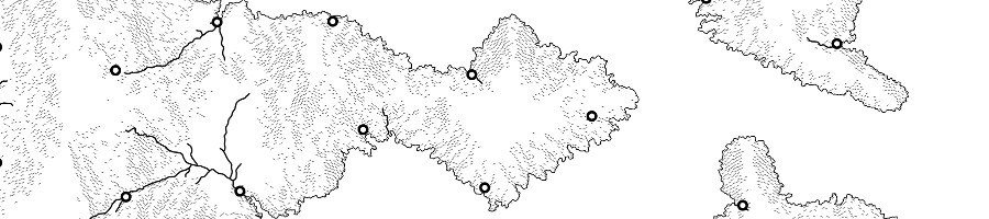
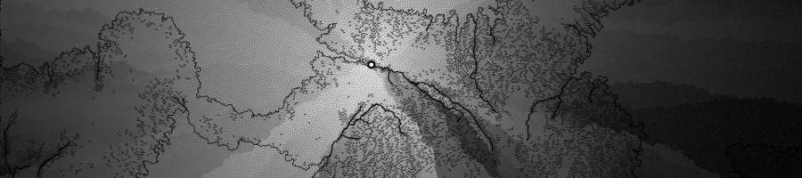
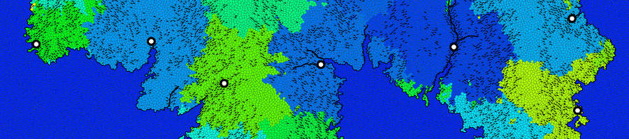
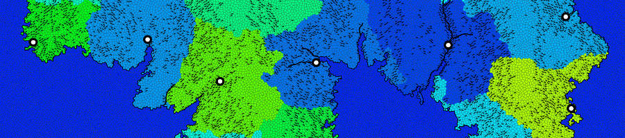
The following images show a variety of maps generated with this program.

Dependencies
There are three dependencies that are required to build this program:
- Python 2.7+ (http://www.python.org/)
- PyCairo graphics library (http://cairographics.org/pycairo/)
- A compiler that supports C++11
Installing PyCairo on Windows
Prebuilt Windows binaries for PyCairo and its dependencies can be obtained by following this guide on installing igraph, which uses PyCairo for drawing. The relevant section is titled "Graph plotting in igraph on Windows".
To check if PyCairo was installed correctly, try importing the module within the Python interpretor:
import cairo
Installation
This program uses the CMake utility to generate the appropriate solution, project, or Makefiles for your system. The following commands can be executed in the root directory of the project to generate a build system for your machine:
mkdir build && cd build
cmake ..
Once successfully built, the program will be located in the
build/ directory.
Running the Map Generator
The map generator is a command line tool and can be invoked with the command:
./map_generator [OPTIONS]
A set of options can be displayed with the --help flag:
>>> ./map_generator --help

Usage: map_generation [-hv] [-s <uint>] [--timeseed] [-r <float>] [-o filename]
[<file>] [-e <float>] [--erosion-steps=<int>] [-c <int>] [-t <int>]
[--size=<widthpx:heightpx>] [--draw-scale=<float>] [--no-slopes] [--no-rivers]
[--no-contour] [--no-borders] [--no-cities] [--no-towns] [--no-labels]
[--no-arealabels] [--drawing-supported]

Options:

  -h, --help                     display this help and exit
  -s, --seed=<uint>              set random generator seed
  --timeseed                     set seed from system time
  -r, --resolution=<float>       level of map detail
  -o, --output=filename          output file
  <file>                         output file
  -e, --erosion-amount=<float>   erosion amount
  --erosion-steps=<int>          number of erosion iterations
  -c, --cities=<int>             number of generated cities
  -t, --towns=<int>              number of generated towns
  --size=<widthpx:heightpx>      set output image size
  --draw-scale=<float>           set scale of drawn lines/points
  --no-slopes                    disable slope drawing
  --no-rivers                    disable river drawing
  --no-contour                   disable contour drawing
  --no-borders                   disable border drawing
  --no-cities                    disable city drawing
  --no-towns                     disable town drawing
  --no-labels                    disable label drawing
  --no-arealabels                disable area label drawing
  --drawing-supported            display whether drawing is supported and exit
  -v, --verbose                  output additional information to stdout
Example:
./map_generation.exe -v --timeseed -r 0.08 -o fantasy_map.png
Leaving the options blank will generate a high quality map with resolution
1920x1080to the file output.png.
Map Generation Process
The map generation process involves the generation of irregular grids, the generation of terrain, the generation of city and towns locations, and their borders, and the generation a label placements.
Generating Irregular Grids
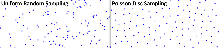
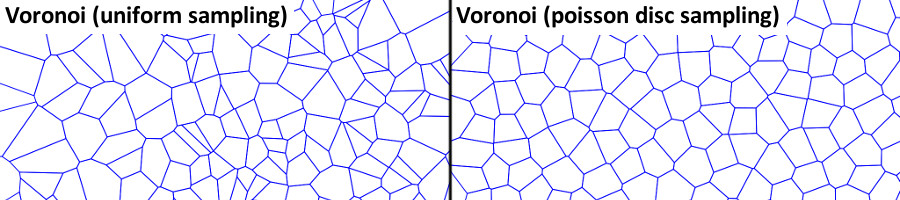
A Poisson disc sampler generates a set of random points with the property that no two points are within a set radius of eachother.
The set of points are triangulated in a Delaunay triangulation. The triangulation is stored in a doubly connected edge list (DCEL) data structure.
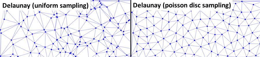
The dual of the Delaunay triangulation is computed to produce a Voronoi diagram, which is also stored as a DCEL.
Each vertex in the Delaunay triangulation becomes a face in the Voronoi diagram, and each triangle in the Delaunay triangulation becomes a vertex in the Voronoi diagram. A triangle is transformed into a vertex by fitting a circle to the three triangle vertices and setting the circle's center as the position of a Voronoi vertex. The following image displays the relationship between a Delaunay triangulation and a Voronoi diagram.
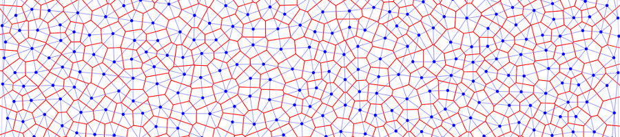
The vertices in the Voronoi diagram will be used as the nodes in an irregular grid. Note that each node has exactly three neighbours.
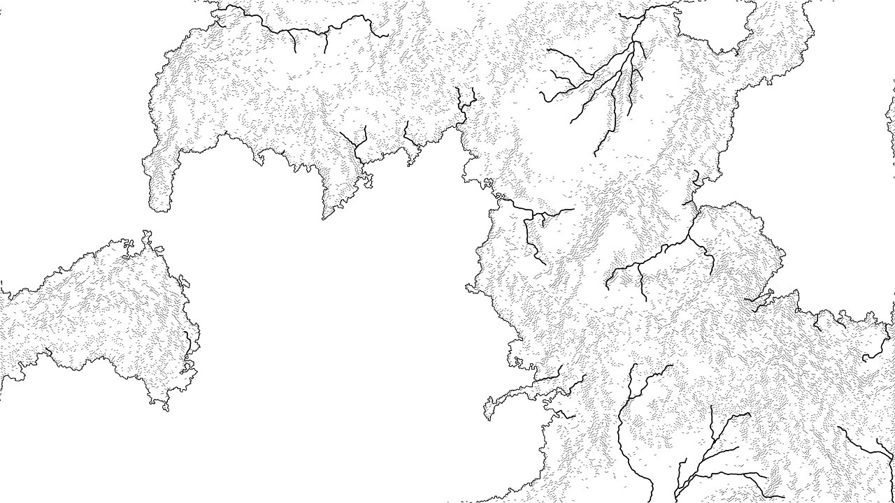
Generating Terrain
An initial height map is generated using a set of primitives:
- addHill - Create a rounded hill where height falls off smoothly
- addCone - Create a cone where height falls off linearly
- addSlope - Create a slope gradient that runs parallel to a line
and a set of operations:
- normalize - Normalize the height map values to [0,1]
- round - Round height map features by normalizing and taking the square root of the height values
- relax - Replace height values with the average of their neighbours
- setSeaLevel - Translate the height map so that the new sea level is at zero
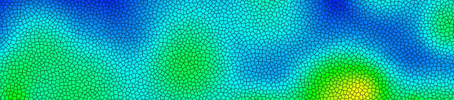
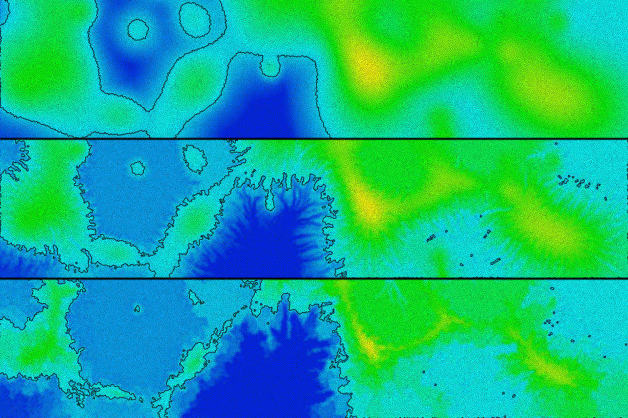
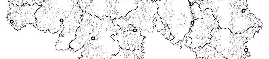
Contour lines are generated from the Voronoi edges. If a contour line is generated for some elevation \(h\), a Voronoi edge will be included in the countour if one of its adjacent faces has a height less than \(h\) while the other has a height greater than or equal to \(h\).
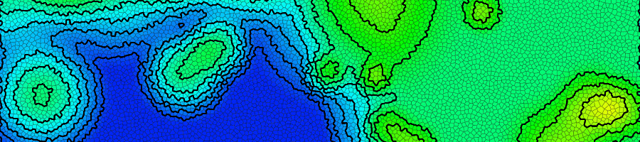
A flow map is generated by tracing the route that water would flow over the map. At each point on the grid, a path must be traced downhill to the edge of the map. This means that there can be no sinks or depressions within the height map. Depressions are filled by using the Planchon-Darboux Algorithm to ensure that a path to the edge of the map exists for all grid points.
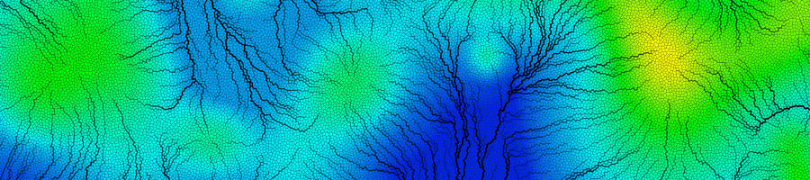
The height map is then eroded by using the flow map data and terrain slope data.
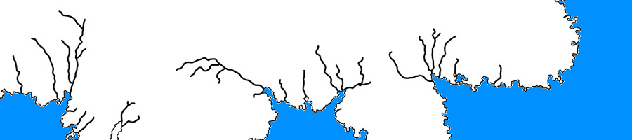
Paths representing rivers are generated at points where the amount of flux (river current) is above some threshold. The path of the river follows the flow map until it reaches a coastline or the edge of the map.
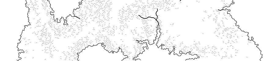
The height map is shaded based upon the horizontal component of the slope. Short strokes are drawn at faces where the slope is above some threshold. Strokes pointing upwards from left to right are drawn if the height map is sloping upward from left to right, and strokes pointing downward from left to right are drawn if the height map is sloping downward from left to right.
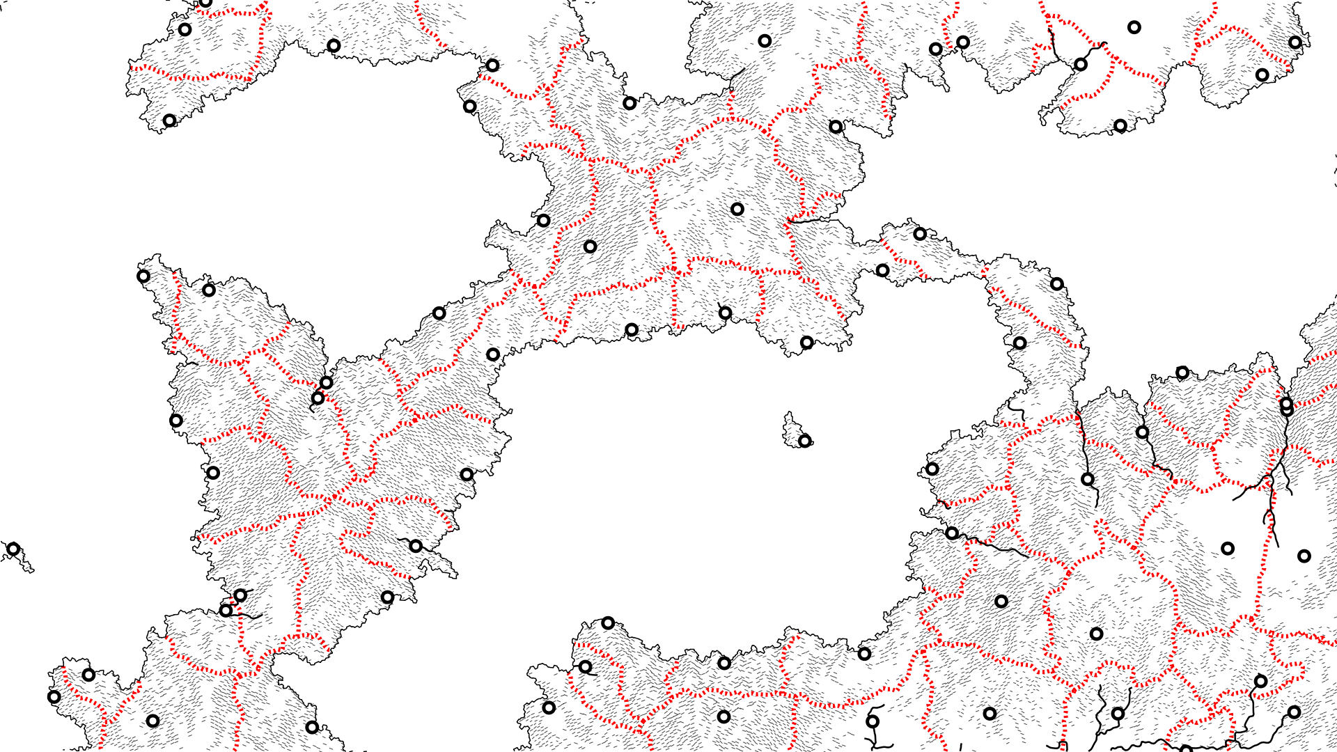
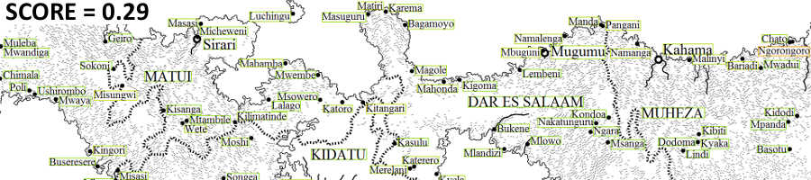
Generating Cities and Borders
City score values are computed before the placement of a city and have a bonus at locations where there is a high flux value and a penalty at locations that are too close to other cities or too close to the edge of the map.
Cities are placed at locations where the city score value is at a maximum.
For each city, the movement cost is calculated for each tile (Voronoi face). Movement costs are based on horizontal and vertical distance, amount of flux (crossing rivers), and transitioning from land to sea (or sea to land).
The tiles are then divided amongst the cities depending on who has the lowest movement cost for the tile.
This method tends to create jagged borders and disjointed territories. The territories are cleaned up by smoothing the edges and by instating a rule that a city territory must contain the city and be a contiguous region.
Borders are then generated around the city territories.
Towns can be added to the map by using the same process that is used to generate city locations. Towns are contained within the city territories and are not involved in territory/border generation.
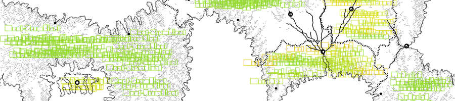
Generating Label Positions
The simulated annealing automated label placement system is based on methods described in the General Cartographic Labeling Algorithm paper.
There are two types of labels that will need to be generated: marker labels that label city and town markers, and area labels that label the city territories.
The labeling process begins by generating candidate label positions for the marker and area labels and calculating a base score for each label.
Marker label candidates are generated around a city or town marker. The calculated scores depend on orientation about the marker, how many river, border, and contour lines the label overlaps, whether the label overlaps another marker, and whether the marker is contained within the map.
Area label candidates are generated within territory boundaries. The calculated scores are similar to the marker label scores except that the orientation score is based upon how much of the label is contained within the territory that it names and how close the center of the label is to the centroid of the territory.
The number of area label candidates is then narrowed down by selecting only the candidates with the best scores.
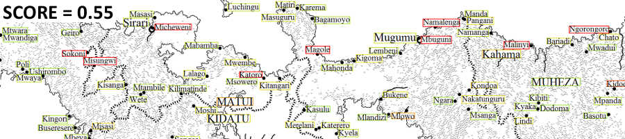
After all candidates for the marker and area labels have been generated, the final label candidates are selected by running the following simulated annealing algorithm:
1. Initialize the label configuration by selecting a candidate randomly for each label.
2. Initialize the "temperature" T to an initial high value.
3. Repeat until the rate of improvement falls below some threshold:
    a) Decrease T according to an annealing schedule.
    b) Chose a label randomly and randomly select a new candidate.
    c) Compute ΔE, the change in label configuration score caused by
       selecting a new label candidate.
    d) If the new labeling is worse, undo the candidate change with
       a probability P = 1.0 - exp(ΔE/T).
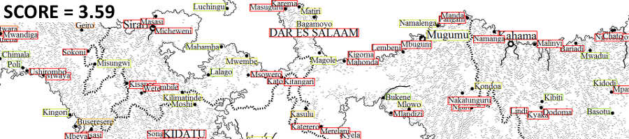
The score of a label configuration is calculated by averaging the base scores of the selected candidates and adding an additional penalty for each set of overlapping candidates.
The initial high value of the temperature \(T\) is set to \(1 / \log(3)\). This value is chosen so that \(P\) evaluates to \(2/3\) when \(\Delta E\) is \(1\).
The loop in step three is terminated when no successful label repositionings are made after \(20 n\) consecutive attempts, where \(n\) is the number of labels, or after some maximum number of temperature changes.
The temperature decreases by \(10\%\) after \(20 n\) label repositioning attemps are made, or if \(5 n\) successful repositioning attemps are made at the same temperature value.
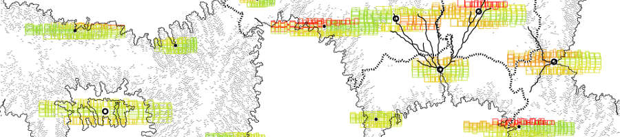
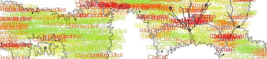
The following set of images show the initial labeling, the labeling halfway through the algorithm, and the final labeling:
References
M. O'Leary, "Generating fantasy maps", Mewo2.com, 2016. [Online]. Available: https://mewo2.com/notes/terrain/. [Accessed: 18- Oct- 2016].
R. Bridson, Fast Poisson Disk Sampling in Arbitrary Dimensions, ACM SIGGRAPH 2007 Sketches Program, 2007.
M. Berg, Computational geometry. Berlin: Springer, 2000.
O. Planchon and F. Darboux, "A fast, simple and versatile algorithm to fill the depressions of digital elevation models", CATENA, vol. 46, no. 2-3, pp. 159-176, 2002.
S. Edmondson, J. Christensen, J. Marks, and S. Shieber, "A General Cartographic Labeling Algorithm", Mitsubishi Electric Research Laboratories, 1996.
J. Christensen, J. Marks and S. Shieber, "An empirical study of algorithms for point-feature label placement", TOG, vol. 14, no. 3, pp. 203-232, 1995.