1 Abstract
This paper presents a simple implementation of a liquid fluid simulation using the method of Smoothed Particle Hydrodynamics (SPH). The SPH model is a Lagrangian method that can be used to model fluid flow by treating each particle as a discrete element of fluid. This paper covers a set of basic equations used to model a fluid, a spatial data structure to accelerate nearest neighbour search, and a method to handle interaction between fluid and solid objects.
2 Introduction
Each SPH fluid particle is treated as a discrete element of fluid. The motion of a fluid particle is influenced by other particles within some finite radius. The amount of influence that a particle has on another depends on the smoothing kernel, which is a single variable function dependent on radius. Since the SPH method is pure Lagrangian, a particle's motion is based on the current acceleration value at a point in time. The acceleration of a particle takes into account the density, pressure, and relative velocities of its surrounding particles.
In order to calculate the density of a particle and the pressure that it exerts on the system, we need to locate its neighbour particles within some radius. To efficiently find neighbours for each particle, a spatial grid is used to refine the search to only particles that are near to each other.
In this implementation, solid objects are modelled in two different ways. The fluid domain boundaries are treated as a set of planes that a particle cannot intersect. These static planes also exert a repulsive force on the particles to keep them away from the boundaries. Dynamic objects are treated as a set of fluid particles whose motion is controlled by an external source. These obstacle particles do not move based on their acceleration, but do keep track of their density and pressure so that other particles can react to them.
3 Implementation
This section provides relevant implementation details for this SPH fluid simulation and will cover the governing equations, the time step calculation, the dynamic spatial grid data structure, the methods of object-fluid interaction, and the user interface.
3.1 Governing Equations
In order to find a particle's acceleration, its density and pressure values must be calculated. The following equation sums the masses of a particle's neighbours weighted by a kernel function.
$$ {\large p_i = \sum_{j}^{ } m_jW_{ij} } $$Where \(p\) is density, \(m\) is mass and \(W\) is the Poly6 smoothing kernel:
$$ {\large W_{ij} = \frac{315}{64\pi h^9}\left( h^2 - r^2 \right)^3 } $$Where \(h\) (chosen as 0.2) is the smoothing radius and \(r\) is the distance between particles. This equation has the advantage of not computing a square root for the distance between particles since the radius is already squared in the equation.
Once a particle's density is found, the pressure can be computed using the ideal gas law:
$$ {\large P = K\left ( p - p_0 \right ) } $$Where \(P\) is pressure, \(p\) is the density of the particle, \(p_0\) is the reference density of the fluid, and \(K\) is a pressure constant. For this implementation, the reference density and pressure constant were both chosen to be 20. In this implementation, the resulting density is set to the reference density if the value is less than the reference density to avoid negative pressures.
Now that the pressure and density of all particles have been calculated, the acceleration of a particle can be computed as:
$$ {\large a_i = -\sum_{j}^{ }\frac{m_j}{m_i}\frac{P_i + P_j} {2p_ip_j}\bigtriangledown W_{ij} \hat{r}_{ij} } $$Where \(a\) is the acceleration, \(P\) is the pressure of the respective particle, \(\hat{r}_{ij}\) is the normalized vector of the position of particle \(j\) to particle \(i\) and \(W\) is the gradient of the following Spiky kernel smoothing function:
$$ {\large \bigtriangledown W_{ij} = -\frac{45}{\pi h^6}\left ( h - r \right )^2 } $$The above acceleration is caused by the mass, density, and pressure of the surrounding particles. To dampen the motion of the system, the velocities of surrounding particles can be taken into account to add a viscosity term to the acceleration:
$$ {\large a_{v_i} = \epsilon \sum_{j}^{ }\frac{m_j}{m_i}\frac{1}{p_j} \left ( v_j - v_i \right ) \bigtriangledown^2 W_{ij} \hat{r}_{ij} } $$Where \(a_v\) is the acceleration due to viscosity, \(\epsilon\) is the viscosity constant (chosen as 0.018 in this implementation), \(v\) is the velocity of the respective particle, and \(W\) is the laplacian of the following viscosity smoothing kernel:
$$ {\large W_{ij} = -\frac{r^3}{2h^3} + \frac{r^2}{h^2} + \frac{h}{2r} - 1 } $$In addition to adding the viscosity term to the particle's acceleration, the acceleration due to the force of gravity is also added.
3.2 Calculating Time Step
The goal of choosing a time step is to choose the largest value such that a particle will move less than one smoothing radius in a single time step. The following equation was used for calculating the next time step in this implementation:
$$ {\large \bigtriangleup t = \max\left ( \frac{Ch}{v_{\text{max}}}, \sqrt{\frac{h}{a_{\text{max}}}}, \frac{Ch}{c_{\text{max}}} \right ) } $$Where \(v_{\text{max}}\) and \(a_{\text{max}}\) are the maximum velocities and accelerations in the particle system, \(c_{\text{max}}\) is the maximum speed of sound, and \(C\) is the Courant safety constant, chosen as 1.0 in this simulation. The safety constant can be set to a higher value for larger timesteps. The speed of sound is calculated with the following equation:
$$ {\large c = \sqrt{\frac{ \gamma P}{p}} } $$Where \(c\) is the speed of sound and \(\gamma\) is the ratio of specific heats, which is set to 1.0 in this simulation.
3.3 Dynamic Spatial Grid
In order to accelerate the nearest neighbour search of all particles, a fixed width spatial grid data structure was implemented. The size of the grid is dynamic, and grid cells only exist where there is fluid. This means that the memory usage of the grid is proportional to the amount of fluid.
Grid cells are contained in a chained hash table according to the following hash function:
$$ {\large \text{hash} = 541i + 79j + 31k } $$Where i, j, k are the respective x, y, z grid indices. The grid cell width is set to one smoothing radius.
Since the particles are only looking up the nearest neighbours within one smoothing radius, we know that at most the particle's cell and 26 cell neighbours need to be looked up. To speed up this process, and to avoid repetitive hash lookups, each grid cell keeps track of its direct neighbours in an array.
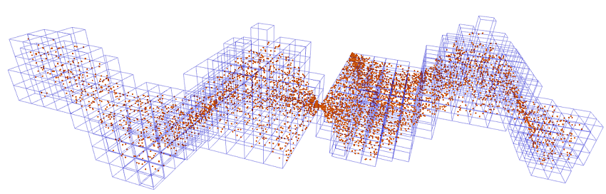
Figure 1. Dynamic Spatial Grid
3.4 Object-Fluid Interaction
Object-fluid interaction is handled in two separate ways depending on the type of object. Static fluid boundaries are handled with planes that the particles cannot intersect. The boundary planes are given a repulsive force in the direction of their normals to push away particles that are too close to the boundary. If a particle hits a boundary, the particle's velocity is adjusted so that it bounces off the surface.
Dynamic objects are handled by constructing the shape with fluid particles. These obstacle particles interact with regular fluid particles as if they were a fluid, except that their motion is controlled by an external force instead of the particle's acceleration. Since obstacle particles are not affected by acceleration, only their pressure and density values are computed. Each obstacle particle is updated for velocity depending on the motion of the object.
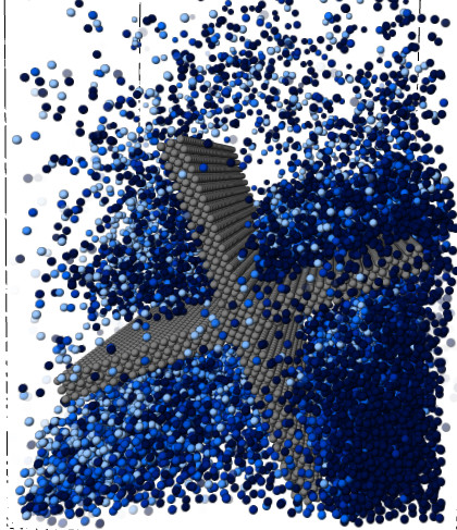
Figure 2. Object-Fluid Interaction
3.5 User Interface
The simulation of a SPH fluid requires the fine-tuning of many constants. Instead of providing a graphical user interface, the simulation is controlled by a Lua script file. This allows the user to change constants and control simulation settings and rendering options while the program is running.
4 Results
To gauge the performance of the simulation, a dam break scenario was created and tested on three datasets of 48958, 98958, and 210504 particles respectively. The dam break consists of three object panels holding back a column of fluid. The centre panel is then lifted to release the fluid into the rest of the simulation domain.
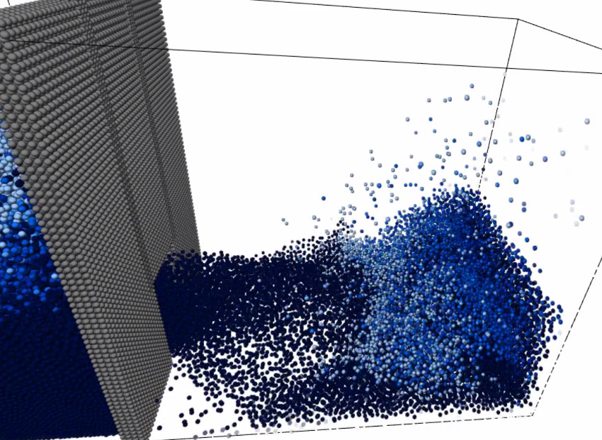
Figure 3. Dam Break Scenario
During testing, five timing metrics were logged for each frame of simulation: total time, nearest neighbour search time, simulation update time, graphics update time, and graphics draw time.
The following table displays the total time results for each test in average minutes per simulation seconds (how long it takes to simulate one second). Each test was ran for 1000 frames at 120 frames per second.
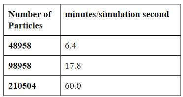
Table 1. Simulation Times
The following table displays the proportion of time spent running the major processes of the simulation.
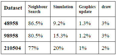
Table 2. Proportion of Simulation Times
We can see that the major bottleneck in this simulation is the nearest neighbour search.
5 Conclusions
Overall, this SPH fluid simulation method was simple to implement and gives graphically believable results for a compressible fluid. Simulation constants were difficult to tweak in order to achieve an incompressible fluid such as water. To model an incompressible fluid, a grid based Navier-Stokes solver may produce more realistic results.
The major bottleneck in simulating this SPH fluid is the nearest neighbour search. To speed up simulation times, effort should be focused on optimizing the spatial grid.
6 References
Roy, Trina. "Physically-Based Fluid Modeling Using Smoothed Particle Hydrodynamics."
Physically-Based
Fluid Modeling Using Smoothed Particle Hydrodynamics. 1 Jan.
1995. Web. 5 Jan. 2015.
<http://www.plunk.org/~trina/thesis/html/thesis_toc.html>.
Cline, David, David Cardon, and Parris K. Egbert. Fluid Flow for the Rest
of Us: Tutorial of the Marker and
Cell Method in Computer Graphics.
N.p.: n.p., n.d. PDF.
Braun, Lucas, and Thomas Lewiner. An Initiation to SPH. Rio De Janeiro,
Brazil: Department of Mathematics,
PUC-Rio, n.d. PDF.
Wang, Lei. "Fluid with Free Surfaces by Smoothed Particle Hydrodynamics."
Lei Wang. Web. 5 Jan. 2015.
<http://web.cse.ohio-state.edu/~whmin/courses/cse788-2011-fall/results/Lei_Wang/788au11.html>.
T, Jakobsen. SPH Survival Kit. N.p.: n.p., n.d. PDF.
Video
The following video is of test footage captured during the building of the program.
Downloads
Download for QT 5.3.0: SPH Fluid Simulation
Download Presentation Slides: Presentation Slides
Source: https://github.com/rlguy/sphfluidsim